Reverse Engineering Crazy Taxi, Part 2

Mar 29, 2026

Reverse Engineering Crazy Taxi, Part 2

Or how I learned to stop worrying and love the cube

This is the second of a series of posts detailing how I put interactive, 3D versions of Crazy Taxi’s levels onto the web. If you haven’t read the first post, I’d highly recommend it, since this builds off many of the ideas developed there.

Part 1: Introduction & archive reversing
Part 2: Reversing shape files (you are here)

In part 1, we covered some basic elements of reverse engineering in order to decode Crazy Taxi’s .all file format, which turned out to be an archive format used to bundle thousands of the game’s asset files. I also stressed a couple lessons I’ve learned while reverse engineering, which I’ll go ahead and recap here:

Take detailed notes as you’re reversing. You never know when that random offset you noticed 2 hours ago will come in handy again.
As early as possible, test your theories with actual code. Writing a quick script that checks your assumption across hundreds of files will save you tons of time compared to manually scanning, and that code can serve as a testbed for further discovery and theorizing.

In this post, we’ll build on these lessons with a couple new techniques in order to puzzle out the .shp file format, which I suspected might have something to do with the game’s 3D models.

What’s in a name?

But why do I think .shp files have anything to do with models? Well for one, .shp looks a lot like the word “shape”, doesn’t it? Admittedly, this is fairly weak evidence by itself, but it was enough to give me my initial hunch and was luckily bolstered by a number of other observations:

Prior to expanding the .all archives, the only .shp file in the game files is called cube0.shp, and cubes are famously a kind of shape. It also seemed roughly the size I’d expect for a cube’s geometry (i.e. small)
Besides cube0.shp, all the other .shp files live in archive files with names like polDC0.all, polDC1.all, etc., whose prefix pol kinda suggests the word “polygon”
The 2,744 .shp files within those archives have names like CZ_train_B.shp, course_4_129.shp, CZ_IMPALA.shp, which all seem like reasonable names for game models

Running with this theory, and assuming cube0.shp indeed contained a cube’s geometry in some Crazy Taxi format, analyzing that file seemed like a great first step to cracking this nut.

Rosetta Cube

Cubes, as you might know, are pretty simple shapes. After the humble triangle, they’re typically the first thing you draw to the screen when writing a renderer or game engine. So the fact that the developers at Acclaim dropped what appears to be a cube written in their proprietary format into our lap makes it something like a Rosetta Stone, since although we don’t know what makes a .shp file tick, we certainly know what to expect from a dang cube.

To inform our investigation into the .shp file, let’s review some standard elements used to store 3D geometry using a well-known, plaintext file format: the Wavefront .obj file. Since .obj files are plaintext, they’re pretty inefficient in terms of filesize, but their simplicity and ease of editing have made them so prolific that even macOS’ builtin file previewer has a full renderer for them:

Previewing a cube using macOS Finder

Now, you don’t need to become an expert in .obj files to understand the rest of this post, but the format’s simplicity makes it a great subject to analyze some of the more universally-used concepts in 3D modeling.

In .obj files, all data is stored as plaintext lines, prefixed by one or two letters to indicate the type of data it is. For our purposes, we’ll only focus on three of these:

Vertex positions: shapes in 3D graphics are made up of points, called vertices, and the most important feature of a vertex is its position. Positions starts with a v and are followed by their $(x, y, z)$ coordinates.
Vertex normals: a vertex normal starts with vn and is also followed by $(x, y, z)$ coordinates, but instead of defining a point, these define a vector, which is math’s version of an arrow. Normal vectors can be somewhat counterintuitive if you haven’t dealt with them before, but basically, they define the direction a surface is facing at some point. This is crucial for adding lighting to a scene, since by knowing which direction a surface faces, we can mathematically “bounce” light off of it and determine how much of that light should reach the viewer.

If you’re struggling to imagine how or why normal vectors are used, imagine we’re trying to render a 3D sphere. As you may know, in computer graphics we represent all 3D shapes as triangles, so our sphere will tragically need to be approximated by some finite number of triangles, making it jagged.

However, by associating a normal vector to each vertex, and by smoothly transitioning between a triangle’s 3 vertex normals, we can associate a nearly-spherical normal vector to every single pixel of that triangle. This is a process called interpolation.

Using some basic math to detect the angle between that interpolated normal and the nearest light lets us calculate how brightly to shade that pixel, ultimately letting us produce the illusion of a smoothly curved surface, despite rendering the same number of triangles as our jagged version. This process is called Phong shading:

Two spheres, the left being rendered with 'flat' surface normals, and the right using radial interpolated normals

Face elements: a face starts with f and is followed by 3 groups of values which describe a triangle. These can come in a couple different formats, but for our purposes, they’ll take this form: f a//m b//n c//o where a, b, and c are position indices (i.e. an index into the list of positions defined above) and m, n, and o are vertex normal indices (ditto for the normals defined above).

With just these elements, we can render and light a 3D shape! To illustrate this (and the .obj format generally), I put together a little visualizer that highlights how each line in an cube.obj file maps to the rendered shape. Mouse over (or tap on) any of the lines below to see how it’s represented in 3D space.

g cube

The main takeaway here is that a shape can be described as a series of triangles, with each vertex in a triangle having some number of attributes (e.g. positions and normal vectors) associated with it. In a bit, we’ll see how other attributes such as color and texture data can be associated with each vertex. And like the positions and normal vectors in our cube.obj example, those attribute values are defined in contiguous arrays by themselves, allowing the triangles to simply be composed of indexes into those arrays. This is so common that these indices are usually just called a model’s “index data”.

Now that we’ve got a sense of how to put a cube in a file, let’s see what Acclaim’s been cooking up.

What’s in the box

At last, here’s cube0.shp. I recommend poking around a bit before continuing, and noting any interesting sections, patterns, or strings that you see.

cube0.shp

Offset

00000000000000100000002000000030000000400000005000000060000000700000008000000090000000a0000000b0000000c0000000d0000000e0000000f000000100000001100000012000000130000001400000015000000160000001700000018000000190000001a0000001b0000001c0000001d0000001e0000001f000000200000002100000022000000230000002400000025000000260000002700000028000000290000002a0000002b0000002c0000002d0000002e0000002f000000300000003100000032000000330000003400000035000000360000003700000038000000390

Bytes

ASCII

Data Inspector:

Bits	uint	int	float
8	-	-	-
16	-	-	-
32	-	-	-

Endianness:

I don’t know how common a practice this is, but when I’m looking at a new binary file format in a hex editor, I’ll often sorta squint my eyes and scroll through it to try to get a feel for how “dense” the data looks at different points. This is useful for identifying the boundaries of different sections of data, since a sequence of 100 floating-point numbers will often look very different than a sequence of 100 16-bit unsigned integers.

Also, for the remainder of this post (and probably future ones), I’ll abbreviate the number formats we’ve been describing as follows: a prefix of either u for an unsigned integer, s for signed integer, or f for floating-point, followed by the bit length. So a 16-bit signed integer is s16, while a 32-bit floating point number is an f32.

To my eyes, there are a couple visibly obvious sections in this file:

0x00 - 0x110:
- Sparsely populated with some probably f32 and maybe u32 values. I’m guessing this is our file header.
0x120 - 0x150:
- Compactly filled with bytes whose integer values are either really big or really small, which I generally would disregard. Maybe they’re f16s?
0x150 - 0x180:
- Starts with some ASCII text that kinda looks like two numbers, followed by some byte data that could be s8
0x180 - 0x1c0:
- Compact array of maybe u16s or s16s
0x1c0 - 0x240:
- Seems to be a mixture of u32s, f32s, u8s, and possibly even some string data (”Format” and even an ASCII-formatted floating-point number??).
0x240 - 0x320:
- Could be u16s or s16s
0x340 - 0x390 (end):
- Seems to be fixed-length strings, two of which reference .tex files that are in some of our .all files, and one that’s… less clear (”mooth { 0x2“)

If you saw some different boundaries, that’s alright! Spoiler alert: my guesses here are not correct.

In any case, there’s clearly a lot more going on here than in the cube.obj file. A perhaps unsurprising reason for this is that unlike cube.obj, Crazy Taxi’s models are textured. That means .shp files have to somehow reference those textures (e.g. the filenames in section 7) and include some coordinates that map the texture to its vertices.

If we scan through section 1, which I guessed was the file header, we first see the f32 value 1.0 which we identified in part 1 as the file’s ”magic number”, or possibly a version number for the .shp format. We then see a handful of small u32ish numbers, and a few more f32s (possibly the shape’s dimensions? world-space position? unclear).

Further down in the header, though, there are some suspiciously familiar u32 values scattered about it. Take a second to look yourself, and see if you can find what I’m talking about. (hint: pay attention to our suspected section boundaries)

It looks like nearly every one of our eyeballed section offsets (e.g. 0x120, 0x180, 0x1c0, etc.) are right in the file’s header, sort of like a table of contents! However unlike in the .all file, these offsets aren’t associated with a string or anything that might identify what they are, which means we’ll need to find another way to identify their purpose. Also, the header includes an offset I didn’t spot in my initial scan, one at 0x160: the data there does look sufficiently different from the preceding ASCII data, so it makes sense that it’s its own section, though it’s not immediately clear to me what it is yet.

Roadblocks and detours

When faced with as many unknowns as we have here, it can be hard to know where to start. A reasonable approach might be to just check out a bunch of different .shp files and look for commonalities and patterns (which I did). I learned a few minor things doing this, such as the header appears to have a fixed size of 0x120 bytes, but nothing terribly helpful.

Another approach might be to start analysing the game’s binary with a tool like Ghidra (which I also did), but at least in this case, digging into the monolithic and symbol-less binary like a GameCube game led to hours of rabbit holes and diversions with no real forward progress. We’ll dig deeper into a Ghidra decompilation of the game in a future post, but for the purposes of cracking the .shp format, it was something of a dead end.

In the end, after spending quite a while spinning my wheels and getting nowhere, I asked for help from Jasper, noclip.website’s developer. And luckily for me, he was able to determine quite a lot of what’s going on here relatively quickly!

That’s because he’s spent years reverse engineering GameCube games and has a seriously impressive working knowledge of that system’s graphics architecture. And while I could just copy his findings here verbatim, I think that’d be missing a valuable learning opportunity for how a beginner might approach this problem on their own. And besides, it’d make this post rather short, so I won’t be doing that.

Instead, I’d like to take us through a bit of background into how the GameCube’s graphics hardware works, and then try to re-derive his findings from first principles with you all. Then, I’ll review some of what his process actually was, since there’s some great lessons to be learned there too.

A brief history of GCN

The GameCube (or GCN, which was Nintendo’s official abbreviation for the platform) contained a custom graphics chip called the Flipper GPU, which was developed during a time when most commercial GPUs used an architecture called the fixed-function pipeline. This meant that after a program (e.g. a game) uploaded its vertex & texture data to the GPU, the GPU would send that data through a predefined set of operations before drawing the result to the screen. This is in contrast to the more modern regime of using programmable shaders, where the game defines what the GPU does using special programs called shaders, which the GPU can run very efficiently. If you’ve ever played a modern PC game, you’re probably familiar with a loading screen that says “Compiling shaders (1/2000)”; this is the process of turning the shader code into programs compiled for your PC’s particular GPU.

Here’s a slide from a Nintendo keynote titled “NINTENDO GAMECUBE: The Ultimate Video Game Machine” which very broadly outlines the flow of the Flipper GPU’s fixed function pipeline:

The GameCube's fixed function pipeline

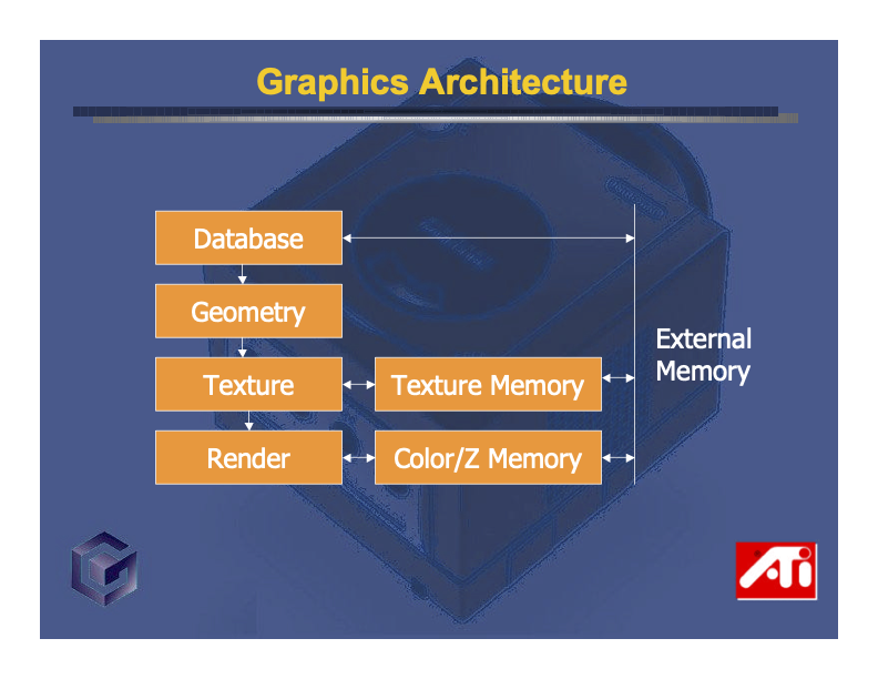
While not particularly illuminating, it does demonstrate a few of the key steps involved in converting model data into pixels.

The way game developers interacted with the Flipper GPU was largely through Nintendo’s GameCube Graphics Library, aka GX. For those interested in a much deeper dive into how this API worked, you can find the original GX manual on the Internet Archive. It’s a surprisingly beginner-friendly and casually written explanation of a lot of 3D graphics basics, and as Jasper pointed out, that’s probably because in 2001 when the GameCube came out, most game developers were beginners to 3D graphics.

In fact, just to underscore how useful finding this manual was, let’s enshrine it as a boldtext reverse engineering lesson: search around for existing documentation! If you find a unique looking project name or error string while poking around a binary, search for it! You’d be surprised how frequently simply searching for a unique error string on GitHub has yielded an accidentally-public repo of proprietary code, or adding “filetype:pdf” to a Google search of a project name resulted in very helpful documentation.

Down the pipeline we go

Anyway, back to the process of convincing GCN to render something. The long and short of it is this:

You submit your model’s data to the GPU in the form of vertex attribute buffers. The Flipper GPU allows each of your model’s vertices to contain up to 12 attributes: 1 position, 1 normal, 2 colors, and 8 texture coordinates, in that order.
In addition to submitting the buffers, you also need to describe which of the 12 attributes you’re using, as well as their format (e.g. f32, s16, etc). This is done by configuring an entry in something called the Vertex Attribute Table, or VAT. For example, a VAT entry might say something like “my attributes contain positions as f32, normals as s16s, and colors as u8 RGB triples”.
- Importantly, for integer types, you can also declare a number of fractional bits, which provides a way of encoding fixed-point (as opposed to floating-point) numbers. We’ll explore this in more detail later.
You submit something Nintendo calls a Display List (or DL) to the GPU. A DL contains commands for the GPU, which can be either a draw call (e.g. “draw some triangles” or “draw some lines”), or a register command that configures part of the fixed-function pipeline (e.g. “use this transform matrix” or “turn on fog with these parameters”).
The GPU sends the DL down its fixed function pipeline and ultimately draws pixels onto the screen.

Now that we know the basics of what GCN expects from Crazy Taxi in order to draw a cube (namely, some vertex attributes and some DL draw calls), let's take another look at `cube0.shp` and see if we can't spot some cubish data.

A return to the cube

To recap what we already know about our file, we have a header occuping the first 0x120 bytes, followed by something like 6 or 7 sections of unknown data:

cube0.shp

Offset

Bytes

ASCII

Data Inspector:

Bits	uint	int	float
8	-	-	-
16	-	-	-
32	-	-	-

Endianness:

Glancing through the sections again, only the section starting at 0x120 looks “dense” enough to contain real-valued numbers like we’d expect from 3D positions, so let’s see if we can find any cube-like position data in there.

First off, how much data are we working with in this section? Because the next section offset in the header is 0x160, it’s tempting to say the section’s 0x160 $-$ 0x120 $=$ 0x40, or 64 in decimal, bytes long. Since we’re expecting the positions of a cube’s vertices, we’d be hoping to see 24 numbers in here (8 points per cube $*$ 3 numbers per point = 24 numbers), which would give us $64/24=2.666...$ bytes per number. Not promising, since $\frac{2}{3}$ of a byte isn’t a workable quantity.

But note that the data starting at 0x150 abruptly changes to bytes which are nearly all ASCII values. While it’s not impossible that our number data coincidentally has ASCII-ish values at times, the consistency here strongly implies that this data is actually a string. However, if it was actually intended to be read as a string, we’d either expect it to have a length prefix (it doesn’t), or be null-terminated with a neat fixed-length block size (it’s not). This pattern occurs a couple times in the .shp file, where we have an abrupt transition from binary data to sloppy ASCII text that’s neither length-prefixed nor a neat fixed-length block.

As such, I think it’s more likely that this is junk data in otherwise empty padding bytes, leftover from whatever dev tooling Acclaim used to create these files. If that’s the case, our section is actually just 0x30 bytes, or 48 in decimal. That’d give us $48/24=2$ bytes per number, which is far more reasonable!

Now, since f16 numbers weren’t an option for GCN vertex attribute values, 2 bytes per number forces our values to be either u16 or s16. And because 3D coordinates generally consist of real-valued numbers that can be negative, let’s assume we’re looking at s16 numbers with a fixed-point fractional component.

The fix is in

I suspect most readers of this are aware of floating-point numbers, which can encode real numbers with an enormous range of precision thanks to their ability to “float” the decimal position. They accomplish this by reserving a portion of the number’s bits for an exponent value, such that $0.1412$ and $141.2$ in floating-point would share the same base value, but would differ in their exponent value.

In contrast, a fixed-point number is a real-valued number encoded in a way that guarantees a, well, fixed degree of decimal precision. But unlike floating-point numbers, that precision isn’t encoded in the number itself, and must be specified by the format. So you wouldn’t just say a 16-bit number is fixed-point, you’d say it’s fixed-point with (for example) 7 integer bits and 9 fractional bits. There’s a common notation for describing this format called Q notation: a Qm.n number consists of $m$ integer bits and $n$ fractional bits, with $m+n$ bits total (or $1+m+n$ bits for signed values). Its value would be the usual base-2 intepretation of its integer component, plus the fractional component scaled by a factor of $\frac{1}{2^n}$ .

Returning to our cube0.shp data, the first two bytes of the 0x120 section are b61a, which as an s16 is $-18,918$ . We ideally want to find the number of fractional bits that scales this to a range close to $[-1, 1]$ , but since the value is so large, the only 16-bit fixed point format able to do that is Q0.15, i.e. one where the entire number is the fractional component. Trying this out, we get:

\frac{-18,918}{2^{15}} = -0.577331543

Which, while not a nice round number like $-0.5$ or $-1$ , does look a bit more promising than $-18,918$ .

What really cemented this theory was when Jasper noticed that if you multiply this result with the second f32 value in the header section (3fddb3d7, which is $1.732$ ), you get:

-0.577331543 * 1.732 = -0.9999382325

Which is almost exactly $-1$ , a number we’d absolutely expect to see in our cube’s vertex data! Perform the same interpretation of the other 23 numbers in the 0x120 section, and add a step to round $\pm0.9999$ to $\pm1$ , and you get this list of values:

-1, -1, -1
1, -1, -1
-1, -1, 1
-1, 1, 1
1, 1, 1
1, 1, -1
-1, 1, -1
1, -1, 1

Which, if plotted as $(x,y,z)$ coordinates does indeed gives us our cube.

To me, this is too neat and tidy to be a coincidence, so I think it’s worth concluding that cube0.shps vertex data starts at 0x120, is composed of s16 fixed-point Q0.15 numbers, which are normalized by a length that’s stored at offset 0x4.

Drawing the rest of the owl

As I mentioned, Jasper determined much of the above pretty quickly, and with some exceptions using pretty similar reasoning. One other useful trick he mentioned using was cutting out the 0x120 section into a new hex editor window and playing with the column width until values sorta “lined up” in a way he expected.

For example, by using a column width of 2 bytes (making each row a single s16), he could quickly see the numbers alternated between just two values. Then, by switching to a column width of 6 (making each row an $(x,y,z)$ coordinate, he saw the 8 positions which resembled the telltale pattern of a cube (i.e. all possible $(x,y,z)$ combinations of those two values).

After determining that the position data was at 0x120, he guessed that many of the other sections might be the other GCN vertex attributes in the order specified by GX: normal vectors, colors 1 and 2, and textures 1 through 8. Using a similar analysis to what we performed on the positions, he noted that the 0x160 section was likely color data, though it’s not immediately clear what format it’s in. Since the ASCII junk starts 12 bytes in, we can assume for now that there’s just 12 bytes of color data.

Then, he noticed the ordering of the u32 offsets in the header starting at 0xcc:

cube0.shp

Offset

00000000 ⋮ 000000cc000000dc000000ec000000fc ⋮ 0000039f

Bytes

(start of file)

0xcc hidden

0x293 hidden

(end of file)

ASCII

⋮

Data Inspector:

Bits	uint	int	float
8	-	-	-
16	-	-	-
32	-	-	-

Endianness:

It starts with 0x120, which we know is our position data, followed by 0x0, then 0x160 which we’re guessing is color data, then another 0x0, and then 0x180 which seems to be some other numeric attribute data. After that, we have enough null bytes to account for (at least) 6 more 0x0 values. Now, wouldn’t it be nice if these 12 values corresponded to the 12 vertex attributes? Then, we’d have:

Corresponding the offset values at 0xcc with the 12 GCN vertex components
No.	Offset	GCN Vertex Attribute
1.	`0x120`	Position
2.	`0x0`	Normal
3.	`0x160`	Color 1
4.	`0x0`	Color 2
5.	`0x180`	Texture 1
6.	`0x0`	Texture 2
...
12.	`0x0`	Texture 8

The sections we know definitely seem to line up, but to be clear, at this point this is just a theory which needs testing. However, if we determine the data at 0x180 is plausibly texture coordinates, that’d be a pretty strong argument in its favor, so let’s take a look.

It’s totally in my Q Zone

Texture coordinates, aka uv coordinates, are so-called because they’re 2D coordinate pairs which traditionally use the letters $(u,v)$ to distinguish them from a position’s $(x,y,z)$ . This post is already far too long to explain them fully, but you can think of them as a way to map a portion of a 2D image (the texture) to each of a 3D object’s triangles. If you’d like to learn more, Wikipedia’s got a great article on this.

One thing to know about uv coordinates is that both of their components tend to be normalized between $[0, 1]$ . So, let’s see if we find a fixed-point format that converts the data at 0x180, which I’m assuming are u16s, into values between $[0, 1]$ . I made a little interactive widget that lets you explore these formats: try changing the number of fractional bits vs. integer bits to fix the values into our expected uv range.

Fixed-point Calculator Q notation: Q16.0

Hex	Binary	Fixed-point Q16.0
0x0001	0000000000000001	1
0x00fe	0000000011111110	254
0x0001	0000000000000001	1
0x0080	0000000010000000	128
0x0001	0000000000000001	1
0x007d	0000000001111101	125
0x0001	0000000000000001	1
0x0001	0000000000000001	1

It looks like using Q8.8 yields the best results, with numbers that range from $[0.0039, 0.9921]$ . Now, eagle-eyed readers will recognize that this is not $[0, 1]$ , but it is close enough that I’d call this a pretty likely theory. Moreover, if we count off our $(u, v)$ pairs and do a little rounding, we end up with these coordinates:

$(0, 1)$
$(0, 0.5)$
$(0.5, 0)$
$(0.5, 0)$
$(0, 0)$

Which yields points that are rather neatly distributed in the uv coordinate space! Even with the rounding, it’s pretty unlikely that we’d get numbers this neat by happenstance, so I’d say our theory that the 0x180 data are texture coordinates passes the sniff test.

Which also means our grander theory that each header offset at 0xcc points to a vertex attribute stream passes muster, so let’s test it with some parsing code. Again, I’m using the lovely Rust library deku to turn our struct into something that can parse binary data:

#[derive(DekuRead)]
#[deku(endian = "big")]
pub struct ShpHeader {
    #[deku(assert_eq = "1.0")]
    pub version: f32,
    unk_block1: [u8; 0xc8], // abbreviated
    // vertex attributes
    pub pos_offset: u32,
    pub norm_offset: u32,
    pub clr_offsets: [u32; 2],
    pub tex_offsets: [u32; 8],
    padding0: [u8; 0x14], // seems to be just zero-padding
    // final four offsets
    pub unk_offset0: u32,
    pub pos_offset_dupe: u32,
    pub unk_offset1: u32,
    pub texture_list_offset: u32,
}

Note that for brevity’s sake, I abbreviated a large section of unknown data between version and pos_offset into a block of 0xc8 bytes. When I was actually working on this, I listed about 20 unk fields in that section which we’ll return to in the next post. Also, the header ends with four other offset values, one of which seems to be the same value as pos_offset and another goes to the list of texture names, so I noted those in the field names.

Keeping it on the DL

Thus far, our theorized .shp format accounts for the 12 possible vertex attribute streams allowed in rendering a model on GCN: positions, normals, colors, and texture coordinates. It also has identified a list of texture names that probably correspond to those texture coordinates. But we’re still missing a key ingredient: the draw call itself. So let’s dig a bit deeper into what GCN draw calls look like.

As a reminder, draw calls are submitted to the GX library in the form of Display Lists (DLs). And luckily for us, the GX manual specifies the DL format precisely!

DLs start with a header byte whose first 5 bits identify the type of call, and whose latter 3 bits are the vertex data’s Vertex Attribute Table (VAT) index. You can think of this header byte as a bitwise OR of the two values: CALL_TYPE | VAT_INDEX. And as we covered earlier, the VAT entry at VAT_INDEX specifies how many of the 12 attributes we’re using in our vertex data; let’s call that number $a$ .

After the header byte is a u16 representing the number of vertices; let’s call this $v$ . Then, we have a stream of $a*v$ indices: one per attribute, per vertex.

If you’re familiar with more common 3D graphics APIs, this might strike you as unusual. That’s because pretty much every other API expects a vertex to provide a single index that’s used across all its attribute buffers, whereas GCN allows each of the vertex’s attribute indices to differ.

The GCN approach provides one clear advantage: smaller attribute buffers.

Suppose 3 vertices have different positions, $P_0, P_1, P_2$ , but use the same color value, $C_0$ . In a modern API, because each vertex has a different position, the indices must also be different, and thus the color attribute buffer would need 3 duplicate copies of $C_0$ for the indices to line up.

But in GCN, the color buffer can just contain the single $C_0$ value, and each vertex color index can reference it separately from the positions.

Pretty early on, Jasper spotted that the data starting at 0x240 looked a lot like DL data:

cube0.shp

Offset

00000000 ⋮ 000002400000025000000260000002700000028000000290000002a0000002b0000002c0000002d0000002e0000002f000000300000003100000032000000330 ⋮ 0000039f

Bytes

(start of file)

0x240 hidden

0x5f hidden

(end of file)

ASCII

⋮

Data Inspector:

Bits	uint	int	float
8	-	-	-
16	-	-	-
32	-	-	-

Endianness:

Initially, this sorta looks like u16 index data, since visually the byte values are somewhat small and increase sequentially. But these values are only small if read as little-endian values, which wouldn’t fit the rest of the file (or the GCN architecture, for that matter). What if instead this was a DL, and thus all of the u16s are offset by the 1 header byte? That’d give us small and sequential big-endian values starting at 0x241.

Cue some GCN-specific knowledge: one of the more common types of draw calls, GX_DRAW_TRIANGLES, has a starting byte equal to 0x90. If we suppose that cube0.shp uses the VAT index 0x03, then a GX_DRAW_TRIANGLES DL would start with 0x93. Then, interpreting the next two bytes as a u16 gives us a vertex count of $v=24$ , and every other 2-byte value reads as an index-like low u16 value.

So let’s do some back-of-the-napkin math here. We know that we have $a=3$ attributes (one for each section we’ve identified: position, color, and texture coordinates), so we’d expect to see $a * v = 3 * 24 = 72$ indices after the first three bytes. At 2 bytes per u16 index, that means $72 * 2 = 144$ bytes. And, adding 144 bytes to our starting offset of 0x240, plus the “header” section of three bytes, gives us a predicted ending offset at 0x2d3, which is just about exactly where the stream of indices ends! So it’s seemingly quite likely that we’ve got a GX_DRAW_TRIANGLES DL command here.

And interestingly, looking ahead to offset 0x2e0, it looks like there’s yet another GX_DRAW_TRIANGLES DL, and the math works out similarly well there.

Putting this all together, it seems that the data starting at 0x240 is a series of DLs that continue all the way until the texture_list_offset section at 0x340 begins. With this observation, we can put a name to another of the offset fields:

#[derive(DekuRead)]
#[deku(endian = "big")]
pub struct ShpHeader {
    #[deku(assert_eq = "1.0")]
    pub version: f32,
    unk_block1: [u8; 0xc8], // abbreviated
    // vertex attributes
    pub pos_offset: u32,
    pub norm_offset: u32,
    pub clr_offsets: [u32; 2],
    pub tex_offsets: [u32; 8],
    padding0: [u8; 0x14], // seems to be just zero-padding
    // final four offsets
    pub unk_offset0: u32,
    pub pos_offset_dupe: u32,
    pub display_list_offset: u32, // new!
    pub texture_list_offset: u32,
}

Just show us the cube man

Ok, so this post about rendering 3D objects in Crazy Taxi has turned out twice as long as I expected and the only 3D thing we’ve seen isn’t even from Crazy Taxi. Sorry about that.

To make an incredibly long story slightly shorter, I’m going to skip the details of how I plugged this .shp data into noclip.website’s GX emulation layer, or the relatively straightforward process of how Jasper figured out the .tex format, and just cut to the cube:

Here it is, the genuine article: cube0.shp rendering as-written directly in the browser. Or rather, it’s a video of it rendering within noclip.

It may not seem that impressive, given that it’s just a handful of points and a pretty boring texture, but much like our work decoding the .all format, these are the necessary building blocks that will eventually let us have the entire Crazy Taxi universe at our fingertips.

Next time, we’ll address the fact that there’s like 2,700 other .shp files that need rendering, and some of them are slightly more complex than a cube.