Dec 15, 2024
I’ve recently gotten very into Leder Games/Cole Wherle’s newest board game, Arcs. It’s a scrappy, clever game about power struggles within a failing interstellar empire, and it’s chock full of deliciously thorny mechanics that lead to interesting decisionmaking.
One of these mechanics is its system of building dice pools. Whenever you send your ships into combat in Arcs, you assemble a dice pool of one die per ship, and resolve the combat in a single roll. What makes this such an interesting bit of decisionmaking is the different types of dice you can pull from for your pool.
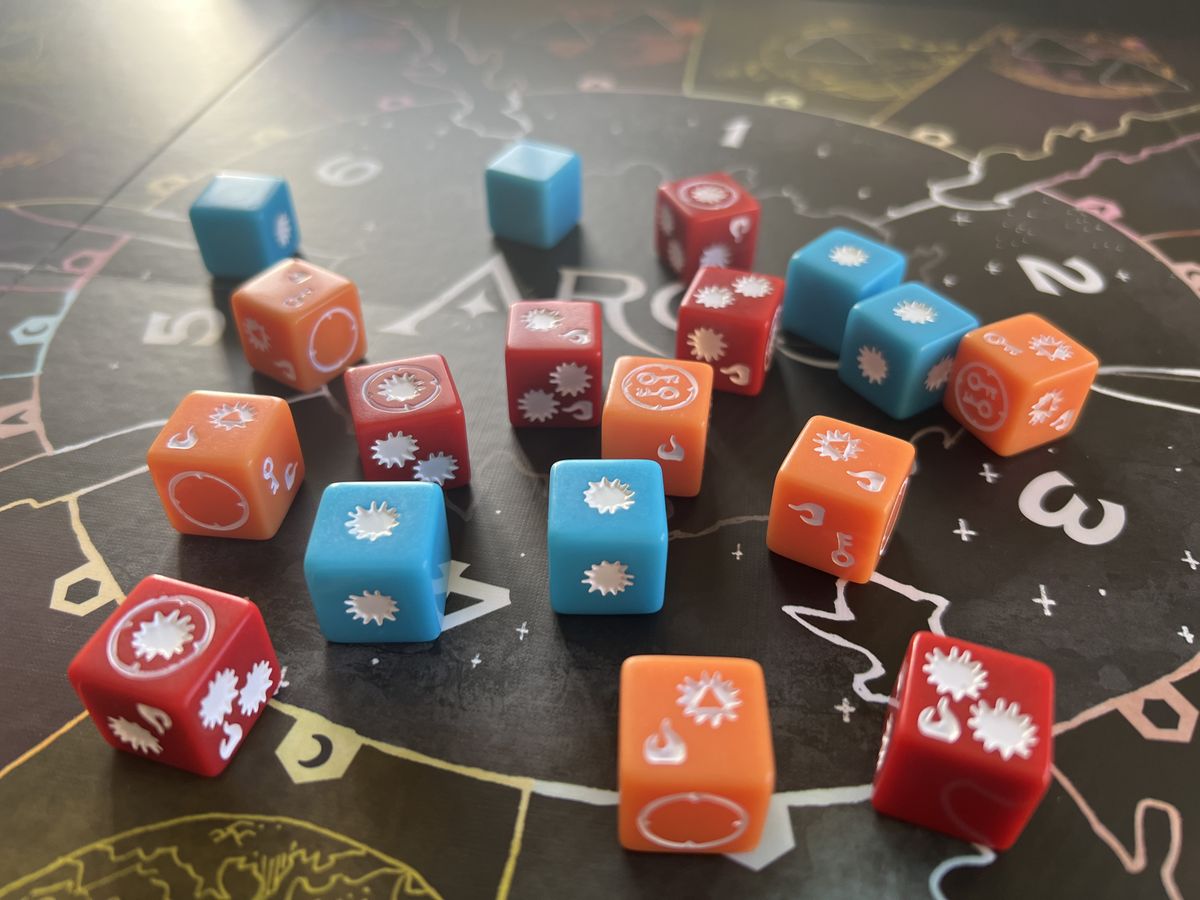
Each die has a different utility and risk profile: blue Skirmish dice are basically a coin flip for whether you’ll score hits against your enemy, and carry no risk of harming your own ships. The red Assault dice can do considerably more damage to the enemy, but with a higher chance of blowing up your fleet with self-hits and intercepts. And the orange Raid dice carry the most risk of self-hits, as well as chances of blowing up enemy buildings (which can be good or bad), but importantly are the only dice which let you roll keys, the game’s way of stealing goodies from your opponent.
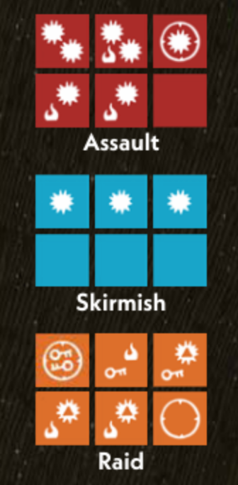
Building your dice pool is an exercise in risk management: how many of your own ships can you afford to blow up to get what you want? With the exception of blue Skirmish dice, the symbols are unevenly allocated over the faces of each die, making for some dramatic dice rolls. For future reference, here’s the layout of each die from the game’s manual:
Now to be clear, I don’t think Cole Wherle intended players to perform exacting calculations of the odds for every dice pool. The gist of the mechanic is that one die is safe, one is risky, and one is real risky, so plan accordingly.
But as a fan of recreational math, I got to wondering: given any assortment of Skirmish, Assault, and Raid dice, what are the odds of rolling any given outcome? For example, suppose I roll 2 Skirmish dice and 2 Assault die, what are the odds of me rolling hits vs self-hits? And as it turns out, what I thought would be a fairly dreadful brute-force statistics problem actually led to some elegant math in unexpected places.
To whet your appetite, here’s a dice pool calculator I wrote using the approach we’re about to cover. Don’t worry if you don’t know Arcs or what a “generating function” is, hopefully that will all make sense by the end of this post.
Dice pool: Generating function: Symbols to compare: 
A simpler case
To start with, let’s analyze the case of rolling a pool of standard six-sided dice and adding up the values. We can consider each die to be a discrete random variable, which means something whose value is randomly determined from a discrete set of values. In this case, those values are , i.e. the number of pips on each die face. Let’s call that random variable for die.
Next, we’d try to model a single roll of this dice pool, which is just the sum of all the random die variables. Since we have dice, let’s call the roll , and thus .
Now, we can finally ask a question like “when rolling 4 dice, what are the odds of rolling a 7?” Or, in a more mathy parlance, what is the value of ’s probability mass function (PMF) ? The problem, of course, is we don’t know what the PMF is yet, so we can’t evaluate it at anything!
Probability mass functions are (in my opinion) terribly named due to a tortured metaphor of probability “densities”, but conceptually they’re actually really simple: they’re just functions which return the probability of getting a value for a given discrete random variable. For example, for a single die, the function is just for all values.
There’s a few ways we can go about calculating the PMF, and Grant Sanderson (aka 3Blue1Brown) has a fantastic video on convolutions which demonstrates some of the traditional approaches. But as I was researching the subject matter, I discovered another way that’s both stranger and more elegant.
Generating functions: a prelude
To spoil the ending a bit, we’ll be using things called generating functions to analyze these dice pool distributions. But I have to admit, when I first learned this approach, it felt extremely bizarre. Generating functions can often seem like total non-sequiters in their applications, and if you’ve never dealt with them before, my goal in this post is to motivate their usage from first principles, and explain why they’re a great fit for this kind of problem. But to quote another Grant Sanderson video:
There’s a time in your life before you understand generating functions, and a time after, and I can’t think of anything that connects them other than a leap of faith.
Back to our roll of dice and its result, . To make things a bit simpler, let’s consider the case of two dice (), and write down all of 36 possible sums of the two rolls:
| Roll | 1 | 2 | 3 | 4 | 5 | 6 |
|---|---|---|---|---|---|---|
| 1 | 2 | 3 | 4 | 5 | 6 | 7 |
| 2 | 3 | 4 | 5 | 6 | 7 | 8 |
| 3 | 4 | 5 | 6 | 7 | 8 | 9 |
| 4 | 5 | 6 | 7 | 8 | 9 | 10 |
| 5 | 6 | 7 | 8 | 9 | 10 | 11 |
| 6 | 7 | 8 | 9 | 10 | 11 | 12 |
As expected, and occur just once to account for the unique rolls (1, 1) and (6, 6) that produce them, and is the most frequent outcome. Since each individual cell of this chart has a chance of occurring, we can simply multiply the number of occurrence of each value by to get the probability of that outcome:
| Roll outcome | # Occurrences | Probability of roll |
|---|---|---|
| 2 | 1 | |
| 3 | 2 | |
| 4 | 3 | |
| 5 | 4 | |
| 6 | 5 | |
| 7 | 6 | |
| 8 | 5 | |
| 9 | 4 | |
| 10 | 3 | |
| 11 | 2 | |
| 12 | 1 |
And hey, just like that we’ve just built a PMF! To calculate the probability of some roll, just look up the outcome and read out its corresponding probability.
Before we proceed, let’s take a step back and generalize the steps we took here. For ease of reference, I’m also going to give each step a name:
- Enumeration: Given the faces on each die, we enumerated the collection of all possible rolls
- Combination: For each possible combination of rolls and :
- We calculated the outcome’s value:
- We calculated the outcome’s probability: (which in our example was just , but worth writing out for later)
- Consolidation: We added together the probabilities of all rolls with equivalent outcomes
Now for the leap of faith. Suppose we wanted a nice, compact, closed-form equation that performs each of these three steps. Luckily, that’s exactly what generating functions allow us to do, though it’s not so clear from the outset how they manage to do it.
Discovering our generating function
Instead of diving into generating functions head-first, let’s approach them a bit more cautiously, and see if we can stumble across one just by trying to design a process that reproduces the 3 above steps: Enumeration, Combination, and Consolidation. For the rest of this section, we’ll be considering the rolls of two standard six-sided dice, and .
First off, Enumeration. What we’re basically looking for is something called a Cartesian product of both die’s set of face values. This would give us all possible pairs of faces from the two dice. One idea that might occur to us is that regular old multiplication can do something like this, which many of us learned as FOIL (First, Out, Inner, Last):
So if we could somehow encode each die as a sum of somethings representing each face, then multiplying those two sums together would give us a giant FOIL’d sum representing every combination of dice faces. For example if we say ’s somethings are , and ’s are , then:
would give us all combinations of ’s and ‘s. But simply setting those somethings to be the face values (e.g. ) clearly wouldn’t work, since we’d just up with the product of two numbers. What else might work?
Well, whatever those somethings are, we know we’re going to be multiplying them together, so let’s recall what we want from our Combination step: the product of two faces should somehow a) add the face values, and b) multiply their respective probabilities. At first, this might seem like something that could only be done in two separate operations. But suppose we encode two outcomes, say and , like this:
What we’ve done here is take the probability of rolling each outcome (), and set it as the coefficient of a single-term polynomial (a.k.a. a monomial) whose degree is equal to the face’s value. Why would we possibly do that? Let’s see what happens when we multiply them together:
Sure enough, we arrive at a new monomial whose coefficient is the probability of the two-dice outcome, and whose degree is equal to the sum of the two rolls. We’ve taken advantage of the unique property that exponents are added when their bases are multiplied to arrive at Combination’s second property, while also multiplying the probability coefficients to get the first property. Pretty convenient!
For the final step, Consolidation, we’d like to add up the probabilities of all outcomes with equivalent values. Luckily enough, our monomial-based encoding scheme handles this for us automatically, since any outcomes with matching degrees will add together naturally:
Now we can start putting the pieces together. Since all faces through of a standard six-sided die have an equal chance of being rolled, it can be described by the polynomial:
This is called a generating function, and although it seems odd to bring this seemingly unrelated polynomial into our problem, remember that we’re just using it to associate probabilities to outcomes. And since, as we’ve seen, multiplying polynomials reproduces our 3 steps, if we multiply by itself we should arrive at a generating function that encodes the probability distribution of rolling two dice:
If we match each exponent-value with the outcome/probability table above, we’ll find that all of the coefficients indeed match the expected probabilities. Moreover, by multiplying our generating function together repeatedly, we can arrive at a compact, closed-form description for an arbitrarily sized dice pool. And so, at last, we can derive the values of the PMF for simply by expanding .
An interlude on
“Cool functions”, I can hear you saying, “but what are they functions of?” And you’re right to be leery. If the coefficients of our function represent probabilities, and the exponents represent dice faces, what meaning does have?
Well in short, it’s just a symbol. When using generating functions to represent our PMF, we’re not really evaluating our for any values of . As Herbert Wilf said in the excellent generatingfunctionology, “a generating function is a clothesline on which we hang up a sequence of numbers for display”. The variable is merely the clothespin holding up the coefficients that we’re interested in, and isn’t necessarily important.
That said, you can definitely treat these critters like real functions and evaulate them at various points to arrive at some really neat insights into your subject. As we’ll see in the next post, there’s some clever evaluation we can do to cheaply pull out our coefficients. A simpler example of this would be to evaluate , which for our generating function above would simply equal the sum of the coefficients (a.k.a. probabilities). And since all probabilities in a distribution must add to equal , we know that .
A more interesting example of this would be . What do you think this might do? Well, for even powers of is just , and for odd powers it’s , so we end up with:
In other words, it subtracts the probability of rolling an odd face from the probability of rolling an even face. In our case, this obviously cancels out to 0, since a 6 sided die has an equal number of even and odd faces. But it also tells us that rolling any number of standard six-sided dice and adding the result has an equal chance of giving an even or odd number, since:
For more on this, be sure to check out Grant Sanderson’s video on generating functions for solving a tough puzzle that I referenced above.
Non-standard dice
So what if we have dice with different numbers of sides, or different allocations of pips? No problem, generating functions got your back. Simply follow the rules of generating functions for PMFs:
- The sum of all coefficients must equal 1
- No coefficients can be negative
With that, let’s try creating the generating function for a 4 sided die with faces :
Since we only have 4 sides, we adjust the coefficients to be , and since one side has 0 pips, we straightforwardly enough assign its probability to , a.k.a. 1. And as you might hope, you can simply multiply with our friend from above to get the generating function for a dice pool with this die and a standard 6 sided die:
Arcs!
We just need one more tool before tackling the dice in Arcs: a way of handling multiple types of pips. In Arcs, each dice can have any number of 5 different symbols. I’ll assign each of them a letter, which will be useful for us going forward:
| Symbol | Name | Letter |
|---|---|---|
| Hit | ||
| Building hit | ||
| Self-hit | ||
| Intecept | ||
| Key |
And for ease of reference, here are the layouts of each die:
How can we represent these? One possiblity might be to create separate generating functions for each type of symbol appearing on each die. So the Assault die would have a hit function, a self-hit function, and an intercept function. But this approach incorrectly treats the different pip types as independent from one another, and would fail to account for the fact that the 1 intercept symbol on Assault dice can only ever be paired with the single hit symbol.
Instead, we make our generating functions multivariate, i.e. they are functions of more than one variable. In this model, each type of die gets its own function on five variables: for Assault dice, for Skirmish, and for Raid:
Note that constant values represent empty faces, and that the probabilities of common terms have been summed together. For brevity’s sake, I’ll refer to these functions by just their capital letters from here on out.
And now we finally have a way to compute the general PMF of any given roll for an arbitrary Arcs dice pool: for a pool of Assault dice, Skirmish dice, and Raid dice, we compute , and then lookup the coefficient of a given roll.
Let’s try a simple example. For a pool with two Assault dice and one Skirmish die, we’d multiply and expand :
As you can see, our (checks notes) “simple” example has give us a pretty unweildy polynomial. But, if you wanted, you could add up all of the coefficients and verify they equal (I certainly did). And although it’s a bit painful to look at, we can fairly easily notice a few things:
- There’s a chance of rolling nothing
- All other possible outcomes include at least one Hit
- The most likely roll is 3 Hits, 2 Self-hits with probability
We can also draw more interesting statistics from this by combing through the terms. For example, the question “what are the chances of rolling more than 3 hits and up to 1 self-hit” is just a matter of adding up the probabilities for every term with a factor of where and .
But as you can see, expanding out and interpreting these polynomials is pretty unweidly, both practically and computationally. Polynomial multiplication is a fairly intensive process, and sifting through the combinatorial explosion of monomials to sum up the coefficients is kind of a nightmare to program. Luckily, as I hinted before, there’s a clever trick we can use to pull out our coefficients in a more efficient and elegant manner. Stay tuned for the next post to learn how!